

In this article I will go through the basics of fitting a choice model to discrete choice experiment data in Q. I’m going to assume you’re familiar with choice experiments and are looking to use Q to analyse data from these surveys.
Selecting a choice model

The first step is to choose the method used to analyse the choice data. The choice is between latent class analysis or hierarchical Bayes. Hierarchical Bayes is more flexible than latent class analysis in modeling the characteristics of each respondent in the survey, so it tends to produce a model that fits the data better. However, latent class analysis is recommended when a segmentation of the respondents is desired.
If you wish to run latent class analysis, select Automate > Browse Online Library > Choice Modeling > Latent Class Analysis. For hierarchical Bayes, select Automate > Browse Online Library > Choice Modeling > Hierarchical Bayes. A new R output called choice.model will appear in the Report tree on the left, with the following controls in the object inspector form on the left (this one is for latent class analysis):
Inputting the design
The next step is to specify the choice experiment design at the Design source control. There are five ways to supply the design:
- Experiment question: supply the design through an Experiment Question in the project.
- Experiment design: supply the design through a choice model design R output in the project (created using Automate > Browse Online Library > Choice Modeling > Experimental Design).
- Sawtooth CHO format: supply the design through a Sawtooth CHO file. You’ll need to upload the CHO file to the project as a data set (first rename it to end in .txt instead of .cho so that it can be recognised by Q).
- Sawtooth dual file format: supply the design through a Sawtooth design file (from the Sawtooth dual file format). Likewise, you’ll need to upload this file to the project as a data set.
- JMP format: supply the design through a JMP design file. Again, you’ll need to upload this file to the project as a data set.
For most of these options, you’ll also need to provide attribute levels through a spreadsheet-style data editor. This is optional for the JMP format if the design file already contains attribute level names. The levels are supplied in columns, with the attribute name in the first row and attribute levels in subsequent rows.
Inputting the respondent data
Whether respondent data needs to be explicitly provided depends on how you supplied the design in the previous step. If an Experiment Question or CHO file was provided, there is no need to separately provide the data, as Experiment Questions and CHO files already contain the choices made by the respondents.
With the other ways of supplying the design, the respondent choices and the task numbers corresponding to these choices need to be provided from variables in the project. Each variable corresponds to a question in the choice experiment. The variables need to be provided in the same order as the questions.
Instead of using respondent data, there is also an option to use simulated data, by changing the Data source setting to Simulated choices from priors. Please see this blog post for more information on using simulated data.
If there are missing responses in the data, Q’s default setting in the Missing data control is to Use partial data. This means that Q will remove questions with missing data for the respondent but keep other questions for analysis. Alternatively, Exclude cases with missing data removes any respondents with missing data, and Error if missing data shows an error message if any missing data is present.
Model settings
The final step is to specify the model settings. There is an option to choose between Latent class analysis or Hierarchical Bayes, so that even though you chose one at the start when creating the output, you can always switch to the other later. If you chose latent class analysis, there is an option to set the number of latent classes and also the number of questions per respondent to leave out for cross-validation.
The more latent classes in the model, the more flexible it is at fitting to the data. However, if there are too many classes, computation time will be long, and the model may be over-fit to the data. For more on latent classes, check out “How to work out the number of classes in latent class analysis“. To work out the amount of overfitting in the data, set Questions left out for cross-validation to be greater than the default of 0. This way, you can compare in-sample and out-of-sample prediction accuracies in the output.
If you choose hierarchical Bayes, you’ll have more options. This is covered in How to Use Hierarchical Bayes for Choice Modeling in Displayr so I won’t go over them here. When you are done with the settings, click on the Calculate button to start the analysis. This may take a few seconds to run or much longer depending on the model specifications and the size of the data.
Filters and Weights
You can apply filter and weights to the output at the bottom of the page, except for hierarchical Bayes, where you cannot apply weights.
Interpreting the output
Shown below is a screenshot from Q of a typical choice model output from a choice experiment on egg preferences. At the top is the title and a subtitle showing the prediction accuracy (out-of-sample accuracy if questions are left out). In the rows of the table are the parameters of the model, which correspond to the attribute levels for categorical attributes, or the attributes themselves for numeric attributes. For each parameter, Q shows a histogram indicating the distribution of its coefficients amongst the respondents. The bars in the histogram are blue and red for positive and negative values respectively.
The last two columns show the mean and standard deviation of the values. A larger magnitude of the mean generally indicates that a parameter is more important, and a larger standard deviation indicates more variation in preference for the parameter’s attribute level. In the example below, the price parameter is completely negative since a high price is worse than a low price, all else being equal. However, there is considerable variation amongst respondents in the value, reflecting differing sensitivities to price.
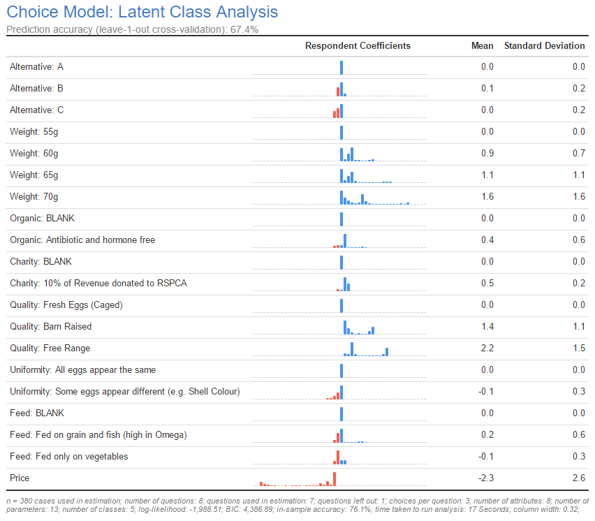
The footer at the bottom of the output contains information about the choice experiment data used and some results from the model such as the log-likelihood and BIC. You can use this for comparison against other model outputs (provided the input data is the same). The in-sample accuracy for when questions are left out for cross-validation can be found in the footer. You should compare this against the out-of-sample accuracy in the subtitle.
Extra features
I have described the process of setting up and running a choice model in Q, but there are still many things that can be done with the choice model output, which are found in the Automate > Browse Online Library > Choice Modeling menu. For example, you can compare and combine outputs into an ensemble model using Compare Models and Ensemble. Diagnostics can be run on the output by highlighting the output and selecting an item from the Automate > Browse Online Library > Choice Modeling > Diagnostics menu, to produce information such as parameter statistics which indicate if there were any issues with parameter estimation. In addition, variables containing respondent coefficients and respondent class memberships can be produced for the output through the Automate > Browse Online Library > Choice Modeling > Save Variable(s) menu.
Find out more about “Using Q” or book a free demo to discover more!